Welcome to Geo Engine Docs
Geo Engine is a cloud-ready geo-spatial data processing platform. This documentation presents the foundations of the system and how to use it.
The Geo Engine
Geo Engine is a cloud-ready geospatial data processing platform. Here, we give an overview of its architecture and describe the main components.
Architecture

Geo Engine consists of the backend and several frontends.
The backend is subdivided into three subcomponents: services, operators, and data types.
Data types specify primitives like feature collections for vector or gridded raster data.
Moreover, it defines plots and basic operations, e.g., projections.
The Operators block contains the processing engine and operators, i.e., source operators, raster- and vector time series processing.
Furthermore, there are raster time series stream adapters, which can be used as building blocks for operators.
The Services block contains protocols, e.g., OGC standard interfaces, as well as Geo Engine specific interfaces.
These can be workflow registration, plot queries, and data upload.
Each of the subcomponents can have additions in Geo Engine Pro, for instance, User Management, which is only available in Geo Engine Pro.
Frontends for the Geo Engine are geoengine-ui for building web applications on top of Geo Engine.
geoengine-python offers a Python library that can be used in Jupyter Notebooks.
3rd party applications like QGIS can access Geo Engine via its OGC interfaces.
All components of Geo Engine are fully containerized and Docker-ready. Geo Engine builds upon several technologies, including GDAL, arrow, Angular, and OpenLayers.
Datasets
A dataset is a loadable unit in Geo Engine.
It is a parameter of a source operator (e.g., a GdalSource) and identifies the data that is loaded.
Geo Engine supports different types of data, reflected by a DataId, which refers to internal datasets and external data.
Internal dataset
An internal dataset is a dataset that is stored in the Geo Engine.
Thus, it is efficiently accessible and can be used in workflows.
The dataset is identified by a DatasetName and contains a DatasetDefinition that describes the data.
The DatasetName is a string that consists of a namespace (optional) and a name, separated by a colon.
For instance, namespace:name or name refer to datasets.
The name can consist of characters (a-Z & A-Z), numbers (0-9), dashes (-) and underscores (_).
External data
An external dataset is a dataset that is not stored in the Geo Engine.
Geo Engine accesses it from a foreign location.
The dataset is identified by an ExternalDataId that consists of a DataProviderId and a LayerId.
While the DatasetProviderId is usually a UUID that identifies the data provider for Geo Engine itself, the LayerId is a string that identifies the layer in the data provider.
The ExternalDataId is a string that consists of a namespace, the DataProviderId and a name, separated by a colon.
The namespace cannot be omitted and is _ for the global namespace.
For instance, _:{uuid}:name or namespace:{uuid}:name refer to datasets.
If the name is a complex string, it can be enclosed by backticks, e.g., namespace:{uuid}:`name with spaces`.
Layers
A layer is a browsable unit in Geo Engine.
In general, it is a named Workflow with additional meta information like a description and a default Colorizer.
Layers are identified by a LayerId, which is usually a UUID.
Every layer can be part of one or more Layer collections.
Layer collections
Layer collections are groups of Layers.
The collections themselves can be grouped inside other collections.
Every layer collection has a name and a description.
Layer collections, just like layers, can be part of one or more other layer collections.
Browsing
Inside Geo Engine’s web interface, you can browse the available layers and layer collections when adding data.
Inside Python, you can use the
ge.layer_collection()
function to get a list of the root collection which contains paths to all underlying layers.
Users and Permission
Geo Engine includes a user management system. Users can either be anonymous or registered. On the first startup, an admin user will be created.
Geo Engine has a Role Based Access Control (RBAC) system.
Users can have different roles and permissions on resources are granted to these roles.
By default, they have a unique role for themselves and either the role anonymous or registered.
The admin user has the role admin.
Geo Engine allows defining permissions for resources like Datasets, Workflows, Layers and Projects.
When a resource is created, the creator gets the Owner permission.
This means they can do everything with the resource, including deleting it and permitting others to use it.
For read-only access, the Read permission is available.
The management of the permissions is done via the Permissions API.
Admin users, i.e. users with the role admin assigned to them, can create new roles and assign them to users.
The management of roles is also done via the Permissions API.
Please refer to the API documentation (TODO: link) for more information.
Alternatively, you can also use our Python library to manage permissions.
Please refer to the Python library documentation for more information.
Example
Let’s say Alice creates a project P.
She automatically gets the Owner permission assigned on the project to her user role.
Then, she adds a Read permission for User Bob.
Before the permission is added, the system checks for the Owner permission on project P.
As Alice is the owner, this operation succeeds.
When Bob tries to access the project P the system checks for the Read permission which again succeeds.
Alice now wants to grant Charly and and Dave the Read permission as well.
Both Charly and Dave have the role Friends of Alice.
She decides to give the permission to the role instead of both users individually.
Both Charly and Dave can now access project P, but Mallory, who does not have the role gets a PermissionDenied error.
When later on Erin gets the role R assigned, she automatically gains access to project P as well.
The complete permission scenario looks like this
- Resources
- project P
- Users
- Alice
- Bob
- Charly
- Dave
- Erin
- Mallory
- Permissions (Role, Resource, Permission)
- Alice, project P, Owner
- Bob, project P, Read
- Friends of Alice, project P, Read
- Roles
- User roles (omitted)
- Friends of Alice
- Charly
- Dave
- Read access allowed
- Alice
- Bob
- Charly
- Dave
- Erin
- Read access denied
- Mallory
API
This chapter introduces the API of Geo Engine.
Workflows
This section introduces the workflow API of Geo Engine.
ResultDescriptor
Call /workflow/{workflowId}/metadata to get the result descriptor of the workflow. It describes the result of the workflow by data type, spatial reference, temporal and spatial extent and some more information that is specific to raster and vector results.
Example response for rasters
{
  "type": "raster",
  "dataType": "U8",
  "spatialReference": "EPSG:4326",
  "measurement": {
    "type": "unitless"
  },
  "time": {
    "start": "2014-01-01T00:00:00.000Z",
    "end": "2014-07-01T00:00:00.000Z"
  },
  "bbox": {
    "upperLeftCoordinate": [-180.0, 90.0],
    "lowerRightCoordinate": [180.0, -90.0]
  }
}
Example response for vectors
{
  "type": "vector",
  "dataType": "MultiPoint",
  "spatialReference": "EPSG:4326",
  "columns": {
    "id": "int",
    "name": "text",
    "value": "float"
  },
  "time": {
    "start": "2014-04-01T00:00:00.000Z",
    "end": "2014-07-01T00:00:00.000Z"
  },
  "bbox": {
    "lowerLeftCoordinate": [3.9662060000000001, 45.9030360000000002],
    "upperRightCoordinate": [19.171284, 51.8473430000000022]
  }
}
Datatypes
This chapter introduces the datatypes of Geo Engine.
Colorizer
A colorizer specifies a mapping between values and pixels/objects of an output image.
Different variants of colorizers perform different kinds of mapping.
In general, there are two families of colorizers: gradient and palette.
Gradients are used to interpolate a continuous spectrum of colors between explicitly stated tuples (breakpoints) of a value and a color.
A palette colorizer on the other hand, is used to generate a discrete set of colors, each mapped to a specific value.
There are three miscellaneous fields in both of the gradient colorizers, namely noDataColor, overColor and underColor.
The field noDataColor is used for all missing, NaN or no data values.
The fields overColor and underColor are used for all overflowing values.
For instance, if there are breakpoints defined from 0 to 10, but a value of -5 or 11 is mapped to a color, the respective field will be chosen instead.
This way, you can specifically highlight values that lie outside of a given range.
For a palette colorizer, there are no overColor and underColor fields.
If a given value does not match any entry in the palette’s definition, it is mapped to the defaultColor.
The noDataColor works in the same manner as in the gradiant variants.
Colors are defined as RGBA arrays, where the first three values refer to red, green and blue and the fourth one to alpha, which means transparency.
The values range from 0 to 255.
For instance, [255, 255, 255, 255] is opaque white and [0, 0, 0, 127] is semi-transparent black.
Linear Gradient
A linear gradient linearly interpolates values within breakpoints of a color table.
For instance, the example below is showing a gradient representing the physical conditions of water at different temperatures.
The gradient is defined between 0.0 and 99.99, where 0.0 is shown as a light blue and 99.99 as blue.
Any value less than 0.0, hence being ice, is shown as white.
Values above 99.99 are shown as a light gray.
Example JSON
{
  "type": "linearGradient",
  "breakpoints": [
    {
      "value": 0.0,
      "color": [204, 229, 255, 255]
    },
    {
      "value": 99.99,
      "color": [0, 0, 255, 255]
    }
  ],
  "noDataColor": [0, 0, 0, 0],
  "overColor": [224, 224, 224, 255],
  "underColor": [255, 255, 255, 255]
}
Logarithmic Gradient
A logarithmic gradient logarithmically interpolates values within breakpoints of a color table and allows only positive values. This colorizer is particularly useful in situations, where the data values increase exponentially and minor changes in the lower numbers would not be recognizable anymore.
Errors
Services report errors that try to use a logarithmic gradient specification with values where value <= 0.
Example JSON
{
  "type": "logarithmicGradient",
  "breakpoints": [
    {
      "value": 1.0,
      "color": [255, 255, 255, 255]
    },
    {
      "value": 100.0,
      "color": [0, 0, 0, 255]
    }
  ],
  "noDataColor": [0, 0, 0, 0],
  "overColor": [0, 0, 0, 255],
  "underColor": [255, 255, 255, 255]
}
Palette
A palette maps values as classes to a certain color.
Unmapped values result in the defaultColor.
Example JSON
{
  "type": "palette",
  "colors": {
    "1": [255, 255, 255, 255],
    "2": [0, 0, 0, 255]
  },
  "noDataColor": [0, 0, 0, 0],
  "defaultColor": [0, 0, 0, 0]
}
RGBA
The RGBA colorizer maps U32 values “as is” to RGBA colors.
8 and 16 bit values are interpreted as grayscale colors.
64 bit values are interpreted as RGBA colors (but loose precision).
Example JSON
{
  "type": "rgba"
}
Measurement
Measurements describe stored data, i.e. what is measured and in which unit.
Unitless
Some values do not have an associated measurement or no information is present.
Example JSON
{
  "type": "unitless"
}
Continuous
The type continuous specifies a continuous variable that is measured in a certain unit.
Example JSON
{
  "type": "continuous",
  "measurement": "Reflectance",
  "unit": "%"
}
Classification
A classification maps numbers to named classes.
Example JSON
{
  "type": "classification",
  "measurement": "Land Cover",
  "classes": {
    "0": "Grassland",
    "1": "Forest",
    "2": "Water"
  }
}
QueryRectangle
A query rectangle defines a multi-dimensional spatial query in Geo Engine. It consists of three parts:
- a two-dimensional spatial bounds (and extent plus its spatial reference system),
- a time interval,
- a spatial resolution.
The spatial bounds behave differently for raster, vector, or plot queries. For raster queries, the spatial bounds define a spatial partition. This means the lower right corner of the spatial bounds is not included in the query. For vector queries, the spatial bounds define a bounding box, i.e., a rectangle where all bounds are included. Plot queries behave like vector queries.
Example JSON
{
  "spatial_bounds": {
    "upper_left_coordinate": {
      "x": 10.0,
      "y": 20.0
    },
    "lower_right_coordinate": {
      "x": 70.0,
      "y": 80.0
    }
  },
  "time_interval": {
    "start": "2010-01-01T00:00:00Z",
    "end": "2011-01-01T00:00:00Z"
  },
  "spatial_resolution": {
    "x": 1.0,
    "y": 1.0
  }
}
RasterBandDescriptor
A raster band descriptor describes a single band of a raster source. The description contains a name and a Measurement.
Example JSON
{
  "name": "NDVI",
  "measurement": {
    "type": "continuous",
    "unit": "NDVI"
  }
}
Raster Data Type
Rasters can have the following data types:
- U8: unsigned 8-bit integer
- I8: signed 8-bit integer
- U16: unsigned 16-bit integer
- I16: signed 16-bit integer
- U32: unsigned 32-bit integer
- I32: signed 32-bit integer
- U64: unsigned 64-bit integer
- I64: signed 64-bit integer
- F32: 32-bit floating-point
- F64: 64-bit floating-point
Example JSON
"U8"
Time Instance
A time instance is a single point in time. It is specified in UTC time zone 0 and has a maximum resolution of milliseconds.
Example JSON
Specifying in ISO 8601:
"2010-01-01T00:00:00Z"
Using the same date as a UNIX timestamp in milliseconds:
1262304000000
Time Interval
A time interval consists of two TimeInstances.
Please be aware, that the interval is defined in close-open semantics.
This means, that the start time is inclusive and the end time of the interval is exclusive.
In mathematical notation, the interval is defined as [start, end).
Example JSON
Specifying in ISO 8601:
{
  "start": "2010-01-01T00:00:00Z",
  "end": "2011-01-01T00:00:00Z"
}
Using the same date as UNIX timestamps in milliseconds:
{
  "start": 1262304000000,
  "end": 1293840000000
}
Time Step
A time step consists of granularity and the number of steps.
For instance, you can specify yearly steps by settings the granularity to Years and the number of steps to 1.
Half-yearly steps can be specified by setting the granularity to Months and the number of steps to 6.
| Parameter | Type | Description | Example Value |
|---|---|---|---|
granularity | TimeGranularity | granularity of the time steps | months |
step | integer | number of time steps | 1 |
TimeGranularity
The granularity of the time steps can take one of the following values.
| Variant | Description |
|---|---|
millis | milliseconds |
seconds | seconds |
minutes | minutes |
hours | hours |
days | days |
months | months |
years | years |
Example JSON
{
  "granularity": "months",
  "step": 1
}
Operators
This chapter introduces the operators of Geo Engine.
Band Neighborhood Agrgegate
The BandNeighborhoodAggregate operator performs a pixel-wise aggregate function over the neighboring bands.
The output is a raster time-series with the same number of bands as the input raster.
The pixel values are replaced by the result of the aggregate function.
This allows e.g. the computation of a moving average over the bands of a raster time-series.
Parameters
| Parameter | Type | Description | Example Value |
|---|---|---|---|
aggregate | NeighborhoodAggregate | The aggrate method | {"type": "average", "windowSize": 3} |
Types
The following describes the types used in the parameters.
NeighborhoodAggregate
There are several types of neighborhood aggregate functions.
Average
This aggregate function computes the average of the neighboring bands.
The windowSize parameter defines the number of bands to consider for the average and must be an odd number.
For the borders, the window is reduced to the available bands.
Example
{
  "type": "average",
  "windowSize": 3
}
FirstDerivative
This aggregate function computes and approximation of the first derivative of the neighboring bands using the central difference method. Given the bands \( x_i \) and the pixel value \( y_i \) the derivative is computed as
\[ f′(x_i) \approx \frac{y_{i+1} − y_{i−1}}{x_{i+1} − x_{i−1}} \]
and forward/backward difference for the endpoints
\[ f′(x_1) \approx \frac{y_2 - y_1}{x_2 - x_1} \]
\[ f′(x_n) \approx \frac{y_n - y_{n-1}}{x_n - x_{n-1}} \]
To compute the distance \( x_{i+1} − x_{i−1} \), a bandDistance parameter is required.
BandDistance
The bandDistance parameter defines the distance between the bands.
Currently, the band distance is assumed to be constant and can be specified in the following way:
{
  "type": "equallySpaced",
  "distance": 1.0
}
Example
{
  "type": "firstDerivative",
  "bandDistance": {
    "type": "equallySpaced",
    "distance": 1.0
  }
}
Inputs
The BandNeighborhoodAggregate operator expects a single raster input .
| Parameter | Type |
|---|---|
source | SingleRasterSource |
Errors
The operation fails if there are not enough bands in the input raster to compute the aggregate function or the number of bands does not match the requirements of the aggregate function.
Example JSON
{
  "type": "BandNeighborhoodAggregate",
  "params": {
    "type": "average",
    "windowSize": 3
  },
  "sources": {
    "raster": {
      "type": "RasterStacker",
      "params": {},
      "sources": {
        "rasters": [
          {
            "type": "GdalSource",
            "params": {
              "data": "sentinel2-b8"
            }
          },
          {
            "type": "GdalSource",
            "params": {
              "data": "sentinel2-b4"
            }
          },
          {
            "type": "GdalSource",
            "params": {
              "data": "sentinel2-b2"
            }
          }
        ]
      }
    }
  }
}
Bandwise Raster Expression
The BandwiseExpression operator performs a pixel-wise mathematical expression on each band of a raster source.
For more details on the expression syntax, see the Expression operator.
Note, that in the BandwiseExpression operator, it is only possible to map one pixel value to another and not reference any other pixels or bands.
The variable name for the pixel value is x.
Parameters
| Parameter | Type | Description | Example Value |
|---|---|---|---|
expression | Expression | Expression script |
|
outputType | RasterDataType | A raster data type for the output |
|
mapNoData | bool | Should NO DATA values be mapped with the expression? Otherwise, they are mapped automatically to NO DATA. |
|
Inputs
The Expression operator expects a single raster input .
| Parameter | Type |
|---|---|
source | SingleRasterSource |
Errors
The parsing of the expression can fail if there are, e.g., syntax errors.
Example JSON
{
  "type": "BandwiseExpression",
  "params": {
    "expression": "ln(1/x)",
    "outputType": "F32",
    "mapNoData": false
  },
  "sources": {
    "raster": {
      "type": "RasterStacker",
      "params": {},
      "sources": {
        "rasters": [
          {
            "type": "GdalSource",
            "params": {
              "data": "sentinel2-b8"
            }
          },
          {
            "type": "GdalSource",
            "params": {
              "data": "sentinel2-b4"
            }
          }
        ]
      }
    }
  }
}
ColumnRangeFilter
The ColumnRangeFilter operator allows filtering FeatureCollections.
Users can define one or more data ranges for a column in the data table that is then filtered.
The filter can be used for numerical as well as textual columns.
Each range is inclusive, i.e., [start, end] includes as well the start as the end.
For instance, you can filter a collection to only include column values that are either in the range 0-10 or 20-30.
Moreover, you can specify the range a to k to dismiss all column values that start with larger letters in the alphabet.
Parameters
| Parameter | Type | Description | Example Value |
|---|---|---|---|
column | string | a column name of the FeatureCollection |
“precipitation” |
ranges | List of either string or number ranges | one or more ranges of either strings or numbers; each range works as an or for the filter |
[[42,43]] |
keepNulls | boolean | should null values be kept or discarded? |
true |
Inputs
The ColumnRangeFilter operator expects exactly one vector input.
| Parameter | Type |
|---|---|
vector | SingleVectorSource |
Errors
If the value in the column parameter is not a column of the feature collection, an error is thrown.
Example JSON
{
  "type": "ColumnRangeFilter",
  "params": {
    "column": "population",
    "ranges": [[1000, 10000]],
    "keepNulls": false
  },
  "sources": {
    "vector": {
      "type": "OgrSource",
      "params": {
        "data": "places",
        "attributeProjection": ["name", "population"]
      }
    }
  }
}
{
  "type": "ColumnRangeFilter",
  "params": {
    "column": "name",
    "ranges": [
      ["a", "k"],
      ["v", "z"]
    ],
    "keepNulls": false
  },
  "sources": {
    "vector": {
      "type": "OgrSource",
      "params": {
        "data": "places",
        "attributeProjection": ["name", "population"]
      }
    }
  }
}
Raster Expression
The Expression operator performs a pixel-wise mathematical expression on one or more bands of a raster source.
The expression is specified as a user-defined script in a very simple language.
The output is a raster time series with the result of the expression and with time intervals that are the same as for the inputs.
Users can specify an output data type.
Internally, the expression is evaluated using floating-point numbers.
An example usage scenario is to calculate NDVI for a red and a near-infrared raster channel.
The expression uses a raster source with two bands, referred to as A and B, and calculates the formula (A - B) / (A + B).
When the temporal resolution is months, our output NDVI will also be a monthly time series.
Parameters
| Parameter | Type | Description | Example Value |
|---|---|---|---|
expression | Expression | Expression script |
|
outputType | RasterDataType | A raster data type for the output |
|
outputBand | RasterBandDescriptor | Description about the output |
|
mapNoData | bool | Should NO DATA values be mapped with the expression? Otherwise, they are mapped automatically to NO DATA. |
|
Types
The following describes the types used in the parameters.
Expression
Expressions are simple scripts to perform pixel-wise computations.
One can refer to the raster inputs as A for the first raster band, B for the second, and so on.
Furthermore, expressions can check with A IS NODATA, B IS NODATA, etc. for NO DATA values.
This is important if mapNoData is set to true.
Otherwise, NO DATA values are mapped automatically to the output NO DATA value.
Finally, the value NODATA can be used to output NO DATA.
Users can think of this implicit function signature for, e.g., two inputs:
fn (A: f64, B: f64) -> f64
As a start, expressions contain algebraic operations and mathematical functions.
(A + B) / 2
In addition, branches can be used to check for conditions.
if A IS NODATA {
    B
} else {
    A
}
Function calls can be used to access utility functions.
max(A, 0)
Currently, the following functions are available:
abs(a): absolute valuemin(a, b),min(a, b, c): minimum valuemax(a, b),max(a, b, c): maximum valuesqrt(a): square rootln(a): natural logarithmlog10(a): base 10 logarithmcos(a),sin(a),tan(a),acos(a),asin(a),atan(a): trigonometric functionspi(),e(): mathematical constantsround(a),ceil(a),floor(a): rounding functionsmod(a, b): division remainderto_degrees(a),to_radians(a): conversion to degrees or radians
To generate more complex expressions, it is possible to have variable assignments.
let mean = (A + B) / 2;
let coefficient = 0.357;
mean * coefficient
Note, that all assignments are separated by semicolons. However, the last expression must be without a semicolon.
Inputs
The Expression operator expects one raster input with at most 8 bands.
| Parameter | Type |
|---|---|
source | SingleRasterSource |
Errors
The parsing of the expression can fail if there are, e.g., syntax errors.
Example JSON
{
  "type": "Expression",
  "params": {
    "expression": "(A - B) / (A + B)",
    "outputType": "F32",
    "outputBand": {
      "name": "NDVI",
      "measurement": {
        "type": "continuous",
        "unit": "NDVI"
      }
    },
    "mapNoData": false
  },
  "sources": {
    "raster": {
      "type": "RasterStacker",
      "params": {},
      "sources": {
        "rasters": [
          {
            "type": "GdalSource",
            "params": {
              "data": "sentinel2-b8"
            }
          },
          {
            "type": "GdalSource",
            "params": {
              "data": "sentinel2-b4"
            }
          }
        ]
      }
    }
  }
}
GdalSource
The GdalSource is a source operator that reads raster data using GDAL.
The counterpart for vector data is the OgrSource.
Parameters
| Parameter | Type | Description | Example Value | Default Value |
|---|---|---|---|---|
data | DataId | The id of the data to be loaded |
|
Inputs
None
Errors
If the given dataset does not exist or is not readable, an error is thrown.
Example JSON
{
  "type": "GdalSource",
  "params": {
    "data": "ndvi"
  }
}
Interpolation
The Interpolation operator artificially increases the resolution of a raster by interpolating the values of the input raster.
If the operator is queried with a resolution that is coarser than the input resolution, the interpolation is not applied but the input raster is returned unchanged.
Unless a particular input resolution is specified, the resolution of the input raster is used, if it is known.
Parameters
| Parameter | Type | Description | Example Value |
|---|---|---|---|
interpolation | InterpolationMethod | the interpolation method to be used | “nearestNeighbor” |
inputResolution | InputResolution | the query resolution for the source operator | “source” |
Types
The following describes the types used in the parameters.
InterpolationMethod
The operator supports the following interpolation methods:
| Value | Description |
|---|---|
nearestNeighbor | The value of the nearest neighbor is used. |
biLinear | The value is computed by bilinear interpolation. |
InputResolution
The operator supports the following input resolutions:
| Value | Description |
|---|---|
{"type": "source"} | The resolution of the input raster is used. |
{"type": "value", "x": 0.1, "y": 0.1} | The resolution is specified explicitly. |
Inputs
The Interpolation operator expects exactly one raster input.
| Parameter | Type |
|---|---|
source | SingleRasterSource |
Errors
If the input resolution is set as “source” but the resolution of the input raster is not known, an error will be thrown.
Example JSON
{
  "type": "Raster",
  "operator": {
    "type": "Interpolation",
    "params": {
      "interpolation": "biLinear",
      "inputResolution": {
        "type": "source"
      }
    },
    "sources": {
      "raster": {
        "type": "GdalSource",
        "params": {
          "data": "ndvi"
        }
      }
    }
  }
}
LineSimplification
The LineSimplification operator allows simplifying FeatureCollections of (multi-)lines or (multi-)polygons by removing vertices.
Users can select a simplification algorithm and specify an epsilon for parametrization.
Alternatively, they can omit the epsilon, which results in the epsilon being automatically determined by the query’s spatial resolution.
For instance, you can remove the vertices of a large country polygon for drawing it on a small map. This results in a simpler polygon that is easier to draw and reduces the amount of data that needs to be transferred.
Parameters
| Parameter | Type | Description | Example Value |
|---|---|---|---|
epsilon | (optional) number | Specify the parametrization of the simplification algorith, e.g. the distance threshold for two nodes in Douglas-Peucker. Must be > 0. |
1.0 |
algorithm | douglasPeucker or visvalingam | Select a simplification algorith for being used, e.g. Douglas-Peucker or Visvalingam |
“douglasPeucker” |
Inputs
The LineSimplification operator expects exactly one vector input.
| Parameter | Type |
|---|---|
vector | SingleVectorSource |
Errors
- If
epsilonis set but <= 0, an error is thrown. - If the input is not
MultiPolygonorMultiLineString, an error is thrown.
Example JSON
{
  "type": "LineSimplification",
  "params": {
    "algorithm": "douglasPeucker",
    "epsilon": 1.0
  },
  "sources": {
    "vector": {
      "type": "OgrSource",
      "params": {
        "data": "ne_10m_admin_0_countries"
      }
    }
  }
}
{
  "type": "LineSimplification",
  "params": {
    "algorithm": "visvalingam"
  },
  "sources": {
    "vector": {
      "type": "OgrSource",
      "params": {
        "data": "ne_10m_admin_0_countries"
      }
    }
  }
}
Neighborhood Aggregate
The NeighborhoodAggregate operator computes an aggregate function for a pixel and its neighborhood.
The operator can be defined as a neighborhood matrix with either weights or predefined shapes and an aggregate function.
An example usage scenario is to calculate a Gaussian filter to smoothen or blur an image. For each time step in the raster time series, the operator computes the aggregate for each pixel and its neighborhood.
The output data type is the same as the input data type. As the matrix and the aggregate in- and outputs are defined as floating point values, the internal computation is done as floating point calculations.
Parameters
| Parameter | Type | Description | Example Value |
|---|---|---|---|
neighborhood | Neighborhood | Pixel neighborhood specification |
|
aggregateFunction | AggregateFunction | An aggregate function for a set of values |
|
Types
The following describes the types used in the parameters.
Neighborhood
There are several types of neighborhoods. They define a matrix of weights. The rows and columns of this matrix must be odd.
WeightsMatrix
The weights matrix is defined as an \( n \times m \) matrix of floating point values. It is applied to the pixel and its neighborhood to serve as the input for the aggregate function.
For instance, a vertical derivative filter (a component of a Sobel filter) can be defined like this:
{
  "type": "weightsMatrix",
  "weights": [
    [1.0, 0.0, -1.0],
    [2.0, 0.0, -2.0],
    [1.0, 0.0, -1.0]
  ]
}
The aggregate function should be sum in this case.
Rectangle
The rectangle neighborhood is defined by its shape \( n \times m \).
The result is a weights matrix with all weights set to 1.0.
{
  "type": "rectangle",
  "dimensions": [3, 3]
}
AggregateFunction
The aggregate function computes a single value from a set of values. The following aggregate functions are supported:
sum: The sum of all valuesstandardDeviation: The standard deviation of all values. This ignoresNO DATAvalues.
Inputs
The NeighborhoodAggregate operator expects exactly one raster input.
| Parameter | Type |
|---|---|
source | SingleRasterSource |
Errors
If the neighborhood rows or columns are not positive or odd, an error will be thrown.
Example JSON
{
  "type": "NeighborhoodAggregate",
  "params": {
    "neighborhood": {
      "type": "weightsMatrix",
      "weights": [
        [1.0, 2.0, 3.0],
        [4.0, 5.0, 6.0],
        [7.0, 8.0, 9.0]
      ]
    },
    "aggregateFunction": "sum"
  },
  "sources": {
    "raster": {
      "type": "GdalSource",
      "params": {
        "data": "ndvi"
      }
    }
  }
}
OgrSource
The OgrSource is a source operator that reads vector data using OGR.
The counterpart for raster data is the GdalSource.
Parameters
| Parameter | Type | Description | Example Value | Default Value |
|---|---|---|---|---|
data | DataId | The id of the data to be loaded |
| |
attributeProjection | Array<String> | (Optional) The list of attributes to load. If nothing is specified, all attributes will be loaded. | [“name”, “population”] | |
attributeFilters | Array<AttributeFilter> | (Optional) The list of filters to apply on the attributes of features. Only the features that match all of the filters will be loaded. |
|
Types
The following describes the types used in the parameters.
AttributeFilter
The AttributeFilter defines one or more ranges on the values of an attribute. The ranges include the lower and upper bounds of the range.
| Field | Type | Description | |
|---|---|---|---|
attribute | String | The name of the attribute to filter. | |
ranges | Array<Array<String | Number>> | The list of ranges to filter. | |
keepNulls | bool | (Optional) Specifies whether to keep null/no data entries, defaults to false. |
Inputs
None
Errors
If the given dataset does not exist or is not readable, an error is thrown.
Example JSON
{
  "type": "OgrSource",
  "params": {
    "data": "places",
    "attributeProjection": ["name", "population"],
    "attributeFilters": [
      {
        "attribute": "population",
        "ranges": [[1000, 10000]],
        "keepNulls": false
      }
    ]
  }
}
PointInPolygon
The PointInPolygon operator filters point features of a (multi-)point collection with polygons.
In more detail, the points of each feature are checked against the polygons of the other collection.
If one or more point is included in any polygon’s ring, the feature is included in the output.
For instance, you can filter tree features inside the polygons of a forest. All features, that weren’t inside any forest polygon, are considered either part of another forest or outliers and are thus removed.
Parameters
The operator is parameterless.
Inputs
The PointInPolygon operator expects two vector inputs.
| Parameter | Type |
|---|---|
points | SingleVectorSource |
polygons | SingleVectorSource |
Errors
If the points vector input is not a (multi-)point feature collection, an error is thrown.
If the polygons vector input is not a (multi-)polygon feature collection, an error is thrown.
Example JSON
{
  "type": "PointInPolygon",
  "params": {},
  "sources": {
    "points": {
      "type": "OgrSource",
      "params": {
        "data": "places",
        "attributeProjection": ["name", "population"]
      }
    },
    "polygons": {
      "type": "OgrSource",
      "params": {
        "data": "germany_outline"
      }
    }
  }
}
Rasterization
The Rasterization operator creates a raster from a point vector source.
It offers two options for rasterization: A grid rasterization and a (gaussian) density rasterization (heatmap).
Inputs
The Rasterization operator expects exactly one vector input.
| Parameter | Type |
|---|---|
source | SingleVectorSource |
Parameters
| Parameter | Type | Description | Example Value |
|---|---|---|---|
params | GridOrDensity | The type and parameters for the rasterization to perform. | {"type": "grid", ...} |
GridOrDensity contains a field type which can have the value grid or density for a grid rasterization or density rasterization, respectively.
GridOrDensity has additional fields which are parameters specific to the type of the rasterization. These are described below separately.
Grid Rasterization
| Parameter | Type | Description | Example Value |
|---|---|---|---|
spatialResolution | SpatialResolution | The spatial resolution of the grid/size of the grid cells. | {"x": 10.0, "y": 10.0} |
originCoordinate | Coordinate2D | The origin coordinate to which the grid is aligned. | {"x": 0.0, "y": 0.0} |
gridSizeMode | fixed or relative | The mode how the grid resolution is interpreted. | "fixed" |
Types
The following describes the types used in the grid rasterization parameters.
The parameters spatialResolution and originCoordinate consist of two fields x and y which describe a resolution/position in x/y direction.
For gridSizeMode the two options fixed and relative are available.
Fixed means the spatialResolution is interpreted as a constant grid cell size.
Relative means the spatialResolution is used as a multiplier for a query’s spatial resolution, making the resulting grid size adaptive to the query resolution.
Density Rasterization
| Parameter | Type | Description | Example Value |
|---|---|---|---|
cutoff | number | Defines the cutoff (as percentage of maximum density) down to which a point is taken into account for an output pixel density value | 0.01 |
stddev | number | The standard deviation parameter for the gaussian function. | 1.0 |
The cutoff percentage (must be in [0, 1)) is treated as a hard cutoff point. A larger cutoff percentage leads to faster processing, however it also introduces inaccuracies in the result since points further than the derived radius away from a pixel do not influence its value.
It is meant to be set such that the ignored density values are small enough to not make a visible difference in the resulting raster.
Errors
If the cutoff is not in [0, 1) or the stddev is negative, an error will be thrown.
Example JSON
Grid Rasterization
{
  "type": "Raster",
  "operator": {
    "type": "Rasterization",
    "params": {
      "type": "grid",
      "spatialResolution": {
        "x": 10,
        "y": 10
      },
      "gridSizeMode": "fixed",
      "originCoordinate": {
        "x": 0,
        "y": 0
      }
    },
    "sources": {
      "vector": {
        "type": "OgrSource",
        "params": {
          "data": "ne_10m_ports",
          "attributeProjection": null,
          "attributeFilters": null
        }
      }
    }
  }
}
Density Rasterization
{
  "type": "Raster",
  "operator": {
    "type": "Rasterization",
    "params": {
      "type": "density",
      "cutoff": 0.01,
      "stddev": 1
    },
    "sources": {
      "vector": {
        "type": "OgrSource",
        "params": {
          "data": "ne_10m_ports",
          "attributeProjection": null,
          "attributeFilters": null
        }
      }
    }
  }
}
RasterScaling
The raster scaling operator scales/unscales the values of a raster by a given slope factor and offset. This allows to shrink and expand the value range of the pixel values needed to store a raster. It also allows to shift values to all-positive values and back. We use the GDAL terms of scale and unscale. Raster data is often scaled to reduce memory/storage consumption. To get the “real” raster values the unscale operation is applied. Keep in mind that scaling might reduce the precision of the pixel values. (To actually reduce the size of the raster, use the raster type conversion operator and transform to a smaller datatype after scaling.)
The operator applies the following formulas to every pixel.
For unscaling the formula is: p_new = p_old * slope + offset. The key for this mode is mulSlopeAddOffset.
For scaling the formula is: p_new = (p_old - offset) / slope. The key for this mode is subOffsetDivSlope.
p_old and p_new refer to the old and new pixel value. The slope and offset values are either properties attached to the input raster or a fixed value.
An example for Meteosat Second Generation properties is:
- offset:
msg.calibration_offset - slope:
msg.calibration_slope
Parameters
| Parameter | Type | Description | Example Value |
|---|---|---|---|
slope | SlopeOffsetSelection | the key or value to use for slope | {"type": "metadataKey" "domain": "", "key": "scale" } |
offset | SlopeOffsetSelection | the key or value to use for offset | {"type": "constant" "value": 0.1 } |
scalingMode | mulSlopeAddOffset OR subOffsetDivSlope | select scale or unscale mode | "mulSlopeAddOffset" |
outputMeasurement* | (optional) Measurement | the measurement of the data produced by the operator | {"type": "continuous", "measurement": "Reflectance","unit": "%"} |
* if no outputMeasurement is given, the measurement of the input raster is used.
The RasterScaling operator expects exactly one raster input.
| Parameter | Type |
|---|---|
source | SingleRasterSource |
Types
The following describes the types used in the parameters.
SlopeOffsetSelection
The SlopeOffsetSelection type is used to specify a metadata key or a constant value.
| Value | Description |
|---|---|
{"type": "auto"} * | Use slope and offset from the tiles properties |
{"type": "constant", "value": number} | A constant value. |
{"type": "metadataKey", "domain": string, "key": string} | A metadata key to lookup dynamic values from raster (tile) properties. |
* if set to "auto", the operator will use the values from the decicated (GDAL) raster properties for scale and offset.
Example JSON
{
  "type": "RasterScaling",
  "params": {
    "slope": {
      "type": "metadataKey",
      "domain": "",
      "key": "scale"
    },
    "offset": {
      "type": "constant",
      "value": 1.0
    },
    "outputMeasurement": null,
    "scalingMode": "mulSlopeAddOffset"
  },
  "sources": {
    "raster": {
      "type": "GdalSource",
      "params": {
        "data": "modis-b6"
      }
    }
  }
}
RasterStacker
The RasterStacker stacks all of its inputs into a single raster time-series.
It does so by querying all of its inputs and outputting them by band, space and then time.
The output raster will have as many bands as the sum of all input bands.
The tiles are automatically temporally aligned.
All inputs must have the same data type and spatial reference.
Parameters
| Parameter | Type | Description | Example Value |
|---|---|---|---|
| renameBands | RenameBands | Specification of how to rename the bands to avoid conflicts | { "type": "default" } |
Types
The following describes the types used in the parameters.
RenameBands
The RenameBands type is used to specify how to rename the bands to avoid conflicts.
| Value | Description |
|---|---|
{"type": "default"} | Appends “ (n)“ to the band name with the smallest n that avoids a conflict |
{"type": "suffix", "values": [string]} | Specifies a suffix for each input, to be appended to the band names |
{"type": "rename", "values": [string]} | A list of names for each band of all inputs to be used instead of the original name |
Inputs
The RasterStacker operator supports up to 8 raster inputs.
| Parameter | Type |
|---|---|
rasters | MultipleRasterSources |
Example JSON
{
  "type": "RasterStacker",
  "params": {
    "renameBands": {
      "type": "rename",
      "values": ["ndvi", "ndvi_masked"]
    }
  },
  "sources": {
    "rasters": [
      {
        "type": "GdalSource",
        "params": {
          "data": "ndvi"
        }
      },
      {
        "type": "Expression",
        "params": {
          "expression": "if A > 100 { A } else { 0 }",
          "outputType": "U8",
          "mapNoData": false
        },
        "sources": {
          "a": {
            "type": "GdalSource",
            "params": {
              "data": "ndvi"
            }
          }
        }
      }
    ]
  }
}
RasterTypeConversion
The RasterTypeConversion operator allows changing the data type of raster data.
It transforms all pixels into the new data type.
-
Applying the operator could lead to a loss of precision, e.g., converting a
F32value of3.1to aU8will return a value of3. -
If the old value is not valid in the new type it will clip at the value range of the new type. E.g., converting a
F32value of300.0to aU8will return a value of255.
Parameters
| Parameter | Type | Description | Example Value |
|---|---|---|---|
outputDataType | [RasterDataType] | the output type | “U8” |
The RasterTypeConversion operator expects exactly one raster input.
| Parameter | Type |
|---|---|
source | SingleRasterSource |
Example JSON
{
  "type": "RasterTypeConversion",
  "params": {
    "outputDataType": "U8"
  },
  "sources": {
    "raster": {
      "type": "GdalSource",
      "params": {
        "data": "ndvi"
      }
    }
  }
}
RasterVectorJoin
The RasterVectorJoin operator allows combining a single vector input and multiple raster inputs.
For each raster input, a new column is added to the collection from the vector input.
The new column contains the value of the raster at the location of the vector feature.
For features covering multiple pixels like MultiPoints or MultiPolygons, the value is calculated using an aggregation function selected by the user.
The same is true if the temporal extent of a vector feature covers multiple raster time steps.
More details are described below.
Example:
You have a collection of agricultural fields (Polygons) and a collection of raster images containing each pixel’s monthly NDVI value.
For your application, you want to know the NDVI value of each field.
The RasterVectorJoin operator allows you to combine the vector and raster data and offers multiple spatial and temporal aggregation strategies.
For example, you can use the first aggregation function to get the NDVI value of the first pixel that intersects with each field.
This is useful for exploratory analysis since the computation is very fast.
To calculate the mean NDVI value of all pixels that intersect with the field you should use the mean aggregation function.
Since the NDVI data is a monthly time series, you have to specify the temporal aggregation function as well.
The default is none which will create a new feature for each month.
Other options are first and mean which will calculate the first or mean NDVI value for each field over time.
Inputs
The RasterVectorJoin operator expects one vector input and one or more raster inputs.
| Parameter | Type |
|---|---|
sources | SingleVectorMultipleRasterSources |
Parameters
The RasterVectorJoin operator has the following parameters:
| Parameter | Type | Description | Example Value |
|---|---|---|---|
names | ColumnNames | Specify how the new column names are derived from the raster band names. |
“{“type”: “default}”
|
featureAggregation | first or mean | The aggregation function to use for features covering multiple pixels. |
“first” |
featureAggregationIgnoreNoData | (optional) boolean | Whether to ignore no data values in the aggregation. Defaults to false |
false |
temporalAggregation | none, first or mean | The aggregation function to use for features covering multiple (raster) time steps. |
“none” |
temporalAggregationIgnoreNoData | (optional) boolean | Whether to ignore no data values in the aggregation. Defaults to false |
false |
Types
ColumnNames
The ColumnNames type is used to specify how the new column names are derived from the raster band names.
| Value | Description |
|---|---|
{"type": "default"} | Appends “ (n)“ to the band name with the smallest n that avoids a conflict |
{"type": "suffix", "values": [string]} | Specifies a suffix for each input, to be appended to the band names |
{"type": "rename", "values": [string]} | A list of names for each new column |
Errors
If the length of names is not equal to the number of raster inputs, an error is thrown.
Example JSON
{
  "type": "RasterVectorJoin",
  "params": {
    "names": ["NDVI"],
    "featureAggregation": "first",
    "temporalAggregation": "mean",
    "temporalAggregationIgnoreNoData": true
  },
  "sources": {
    "vector": {
      "type": "OgrSource",
      "params": {
        "data": "places"
      }
    },
    "rasters": [
      {
        "type": "GdalSource",
        "params": {
          "data": "ndvi"
        }
      }
    ]
  }
}
Reprojection
The Reprojection operator reprojects data from one spatial reference system to another.
It accepts exactly one input which can either be a raster or a vector data stream.
The operator produces all data that, after reprojection, is contained in the query rectangle.
Data type specifics
The concrete behavior depends on the data type.
Vector data
The reprojection operator reprojects all coordinates of the features individually. The result contains all features that, after reprojection, are intersected by the query rectangle. If not all coordinates of the vector data stream could be projected, the operator returns an error.
Raster data
To create tiles in the target projection, the operator first loads the corresponding tiles in the source projection. Note, that in order to create one reprojected output tile, it may be necessary to load multiple source tiles. For each output pixel, the operator takes the value of the input pixel nearest to its upper left corner.
In order to obtain precise results but avoid loading too much data, the operators estimate the resolution in which it loads the input raster stream. The estimate is based on the target resolution defined by the query rectangle and the relationship between the length of the diagonal of the query rectangle in both projections. Please refer to the source code for details.
In case a tile, or part of a tile, is not available in the source projection because it is outside of the defined extent, the operator will produce pixels with no data values. If the input raster stream has no no data value defined, the value 0 will be used instead.
Parameters
| Parameter | Type | Description | Example Value |
|---|---|---|---|
targetSpatialReference | String | The srs string (authority:code) of the target spatial reference. | EPSG:4326 |
Inputs
The Reprojection operator expects exactly one raster or vector input.
| Parameter | Type |
|---|---|
source | RasterOrVectorOperator |
Errors
The operator returns an error if the target projection is unknown or if the input data cannot be reprojected.
Example JSON
{
  "type": "Reprojection",
  "params": {
    "targetSpatialReference": "EPSG:4326"
  },
  "sources": {
    "source": {
      "type": "GdalSource",
      "params": {
        "data": "ndvi"
      }
    }
  }
}
TemporalRasterAggregation
The TemporalRasterAggregation aggregates a raster time series into uniform time intervals (windows).
The output is a time series that begins with the first window that contains the start of the query time.
Each time slice has the same length, defined by the window parameter.
The pixel values are computed by aggregating all rasters that are contained in the input and that are valid in the current window using the defined aggregation method.
All output slices that are contained in the query time interval are produced by the operator.
The optional windowReference parameter allows specifying a custom anchor point for the windows.
This is the imagined start from which on the timeline is divided into uniform aggregation windows.
By default, it is 1970-01-01T00:00:00Z which means that windows of, e.g., 1 hour or 1 month will begin at the full hour or the start of the month.
An example usage scenario is to transform a daily raster time series into monthly aggregates.
Here, the query should start at the beginning of the month and the window should be 1 month.
The aggregation method allows calculating, e.g., the maximum or mean value for each pixel.
If we perform a query with time [2021-01-01, 2021-04-01), we would get a time series with three time steps.
If we perform a query with an instant like [2021-01-01, 2021-01-01), we will get a single time step containing the aggregated values for January 2021.
Parameters
| Parameter | Type | Description | Example Value |
|---|---|---|---|
aggregation | Aggregation | method for aggregating pixels | { "type": "max", "ignoreNoData": false} |
window | TimeStep | length of time steps | { "granularity": "Months", "step": 1} |
windowReference | TimeInstance | (Optional) anchor point for the aggregation windows. Default value is 1970-01-01T00:00:00Z | 1970-01-01T00:00:00Z |
outputType | RasterDataType | (Optional) A raster data type for the output. Same as input, if not specified. | U8 |
Types
The following describes the types used in the parameters.
Aggregation
There are different methods that can be used to aggregate the raster time series.
Encountering a no data value makes the aggregation value of a pixel also no data unless the ignoreNoData parameter is set to true.
| Variant | Parameters | Description |
|---|---|---|
min | ignoreNoData: bool | minimum value |
max | ignoreNoData: bool | maximum value |
first | ignoreNoData: bool | first encountered value |
last | ignoreNoData: bool | last encountered value |
mean | ignoreNoData: bool | mean value |
percentileEstimate | ignoreNoData: bool, percentile: number in (0, 1) | computes a percentile estimate using the P² method |
sum | ignoreNoData: bool | sum of the values |
count | ignoreNoData: bool | count the number of values |
Attention: For the variants sum and count, a saturating addition is used.
This means, that if the sum of two values exceeds the maximum value of the data type, the result will be the maximum value of the data type.
Thus, users must be aware to choose a data type that is large enough to hold the result of the aggregation.
Inputs
The TemporalRasterAggregation operator expects exactly one raster input.
| Parameter | Type |
|---|---|
raster | SingleRasterSource |
Errors
If the aggregation method is first, last, or mean and the input raster has no no data value, an error is thrown.
Example JSON
{
  "type": "TemporalRasterAggregation",
  "params": {
    "aggregation": {
      "type": "max",
      "ignoreNoData": false
    },
    "window": {
      "granularity": "Months",
      "step": 1
    },
    "windowReference": "1970-01-01T00:00:00Z",
    "sources": {
      "raster": {
        "type": "GdalSource",
        "params": {
          "data": "ndvi"
        }
      }
    }
  }
}
TimeProjection
The TimeProjection projects vector dataset timestamps to new granularities and ranges.
The output is a new vector dataset with the same geometry and attributes as the input.
However, each time step is projected to a new time range.
Moreover, the QueryRectangle’s temporal extent is enlarged as well to include the projected time range.
An example usage scenario is to transform snapshot observations into yearly time slices.
For instance, animal occurrences are observed at a daily granularity.
If you want to aggregate the data to a yearly granularity, you can use the TimeProjection operator.
This will change the validity of each element in the dataset to the full year where it was observed.
This is, for instance, useful when you want to combine it with raster time series and use different temporal semantics than the originally recorded validities.
Parameters
| Parameter | Type | Description | Example Value |
|---|---|---|---|
step | TimeStep | time granularity and size for the projection |
|
stepReference | TimeInstance | (Optional) an anchor point for the time step |
“2010-01-01T00:00:00Z” |
Inputs
The TimeProjection operator expects exactly one vector input.
| Parameter | Type |
|---|---|
vector | SingleVectorSource |
Errors
If the step is negative, an error is thrown.
Example JSON
{
  "type": "TimeProjection",
  "params": {
    "step": {
      "granularity": "years",
      "step": 1
    }
  },
  "sources": {
    "vector": {
      "type": "OgrSource",
      "params": {
        "data": "ndvi"
      }
    }
  }
}
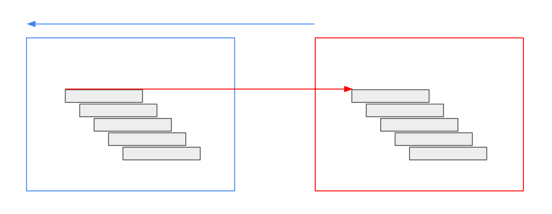
TimeShift
The TimeShift operator allows retrieving data temporally relative to the actual QueryRectangle.
It shifts the query rectangle by a given amount of time and modifies the result data accordingly.
Users have two options for specifying the time shift:
- Relative shift – shift relatively to the query rectangle, e.g., one month or one year to the past. This can be useful for comparing multiple points in time relative to the query rectangle.
- Absolute shift – change query rectangle to a fixed temporal reference, e.g., January 2014. This can be used to compare data in the query rectangle’s time to a fixed point of reference.
The output is either a stream of raster data or a stream of vector data depending on the input.
An example usage scenario is to compare the current time with the previous time of the same raster data.
For instance, a raster source outputs monthly data aggregates of mean temperatures.
If you want to compute the difference between the current month and the previous month, you can use the TimeShift operator.
You will have two workflows.
One is the unmodified temperature raster source.
The other is the same source, shifted by one month.
Then, you can use both workflows as sources of an Expression operator.
Note: This operator modifies the time values of the returned data.
For rasters and vector data, it shifts the time intervals opposite to the time shift specified in the operator.
This is necessary to have only data inside the result that is part of the QueryRectangle’s time interval.
As an example, we shift monthly data by one month to the past.
Our query rectangle points to February.
Then, the operator shifts the query rectangle to January.
The data, originally valid for January, is shifted forward to February again, to fit into the original query rectangle, which is February.
Parameters
| Parameter | Type | Description | Example Value |
|---|---|---|---|
type | relative or absolute | shift relatively or absolute |
“relative” |
Relative
If type is relative, you need to specify the following parameters:
| Parameter | Type | Description | Example Value |
|---|---|---|---|
granularity | TimeGranularity | time granularity and for the shift |
“months” |
value | integer | the size of the step |
-1 |
Absolute
If the type is absolute, you need to specify the following parameters:
| Parameter | Type | Description | Example Value |
|---|---|---|---|
timeInterval | TimeInterval | A fixed shift of the QueryRectangle’s time |
|
Inputs
The TimeShift operator expects either one vector input or one raster input.
| Parameter | Type |
|---|---|
source | SingleRasterOrVectorSource |
Example JSON
{
  "type": "TimeShift",
  "params": {
    "type": "relative",
    "granularity": "months",
    "value": -1
  },
  "sources": {
    "source": {
      "type": "GdalSource",
      "params": {
        "data": "ndvi"
      }
    }
  }
}
{
  "type": "TimeShift",
  "params": {
    "type": "absolute",
    "time_interval": {
      "start": "2010-01-01T00:00:00Z",
      "end": "2010-02-01T00:00:00Z"
    }
  },
  "sources": {
    "source": {
      "type": "GdalSource",
      "params": {
        "data": "ndvi"
      }
    }
  }
}
Vector Expression
The VectorExpression operator performs a feature-wise expression function on a feature collection of a vector source.
The expression is specified as a user-defined script in a very simple language.
The output is a feature collection with the result of the expression and with time intervals that are the same as for the inputs.
Users can either add a new column or replace the geometry column with the outputs of the expression.
Internally, the expression is evaluated using floating-point numbers.
An example usage scenario is to calculate a population density from an area and a population_size column.
The expression uses a feature collection with two columns, referred to with their column names area and a population_size, and calculates the formula area / population_size.
The output feature collection contains the result of the density expression in a new column.
Another example is to calculate the centroid of a polygon geometry.
The expression uses a feature collection with a geometry column and calculates the formula centroid(geom).
The output feature collection contains the result of the centroid expression replacing the original geometries.
Parameters
| Parameter | Type | Description | Example Value |
|---|---|---|---|
expression | Expression | Expression script |
|
inputColumns | Vec<String> | The names of the attributes to generate boxes for. |
|
outputColumn | OutputColumn | An output column name or a geometry type |
|
geometryColumnName | String (optional) | A name for the geometry variable. geom by default. |
|
outputMeasurement | Measurement | Description about the output |
|
Note:
If a name in inputColumns contains any characters other than letters, numbers, and underscores, a canonical variable name has so be used in the expression.
For example, the column name population size has to be referred to as population_size in the expression.
Types
The following describes the types used in the parameters.
Expression
Expressions are simple scripts to perform feature-wise computations.
One can refer to the columns with their name, e.g., area and a population_size.
Furthermore, expressions can check with A IS NODATA, B IS NODATA, etc. for empty or NO DATA values.
Finally, the value NODATA can be used to output empty or NO DATA.
Users can think of this implicit function signature for, e.g., two inputs:
fn (A: f64, B: f64) -> f64
As a start, expressions contain algebraic operations and mathematical functions.
(A + B) / 2
In addition, branches can be used to check for conditions.
if A IS NODATA {
    B
} else {
    A
}
To generate more complex expressions, it is possible to have variable assignments.
let mean = (A + B) / 2;
let coefficient = 0.357;
mean * coefficient
Note, that all assignments are separated by semicolons. However, the last expression must be without a semicolon.
Numbers
Function calls can be used to access utility functions.
max(A, 0)
Currently, the following functions are available:
abs(a): absolute valuemin(a, b),min(a, b, c): minimum valuemax(a, b),max(a, b, c): maximum valuesqrt(a): square rootln(a): natural logarithmlog10(a): base 10 logarithmcos(a),sin(a),tan(a),acos(a),asin(a),atan(a): trigonometric functionspi(),e(): mathematical constantsround(a),ceil(a),floor(a): rounding functionsmod(a, b): division remainderto_degrees(a),to_radians(a): conversion to degrees or radians
Geometries
Geometries can be referred to using the geometryColumnName, which is geom by default.
There are several functions to work with geometries:
centroid(geom): returns the centroid of the geometryarea(geom): returns the area of the geometry
An example expression to calculate the centroid of a geometry is:
centroid(geom)
Inputs
The VectorExpression operator expects one rater input with at most 8 bands.
| Parameter | Type |
|---|---|
vector | SingleVectorSource |
Errors
The parsing of the expression can fail if there are, e.g., syntax errors.
Example JSON
{
  "type": "VectorExpression",
  "params": {
    "inputColumns": ["area", "population_size"],
    "outputColumn": { "type": "column", "value": "density" },
    "expression": "area /  population_size",
    "outputMeasurement": { "type": "unitless" }
  },
  "sources": {
    "vector": {
      "type": "OgrSource",
      "params": {
        "data": "areas"
      }
    }
  }
}
{
  "type": "VectorExpression",
  "params": {
    "inputColumns": [],
    "outputColumn": { "type": "geometry", "value": "MultiPoint" },
    "expression": "centroid(geom)",
    "geometryColumnName": "geom"
  },
  "sources": {
    "vector": {
      "type": "OgrSource",
      "params": {
        "data": "areas"
      }
    }
  }
}
VectorJoin
The VectorJoin operator allows combining multiple vector inputs into a single feature collection.
There are multiple join variants defined, which are described below.
For instance, you want to join tabular data to a point collection of buildings. The point collection contains the geolocation of the buildings and their id. The attribute data collection has the building id and the height information. Combining the two feature collections leads to a single point collection with geolocation and height information.
Parameters
| Parameter | Type | Description | Example Value |
|---|---|---|---|
type | A value of EquiGeoToData, … | The type of join |
“EquiGeoToData” |
EquiGeoToData
| Parameter | Type | Description | Example Value |
|---|---|---|---|
leftColumn | string | The column name of the left input |
“id” |
rightColumn | string | The column name of the right input |
“id” |
rightColumn_suffix | (Optional) string | A value to suffix the right join column to avoid name clashes with the columns of the left input. If nothing is specified, the default value is right. |
“right” |
Inputs
The VectorJoin operator expects two vector inputs.
| Parameter | Type |
|---|---|
left | SingleVectorSource |
right | SingleVectorSource |
Errors
If the value in the left parameter is not a column of the left feature collection, an error is thrown.
If the value in the right parameter is not a column of the right feature collection, an error is thrown.
EquiGeoToData
If the left input is not a geo data collection, an error is thrown.
If the right input is not a (non-geo) data collection, an error is thrown.
Example JSON
{
  "type": "VectorJoin",
  "params": {
    "type": "EquiGeoToData",
    "leftColumn": "id",
    "rightColumn": "id",
    "rightColumnSuffix": "_other"
  },
  "sources": {
    "points": {
      "type": "OgrSource",
      "params": {
        "data": "places",
        "attributeProjection": ["name", "population"]
      }
    },
    "polygons": {
      "type": "OgrSource",
      "params": {
        "data": "germany_outline"
      }
    }
  }
}
VisualPointClustering
The VisualPointClustering is a clustering operator for point collections that removes clutter and preserves the spatial structure of the input.
The output is a point collection with a count and radius attribute.
The operator utilizes the input resolution of the query to determine when points, being displayed as circles, would overlap.
Moreover, it allows aggregating non-geo attributes to preserve the other columns of the input.
For more information on the algorithm, cf. the paper Beilschmidt, C. et al.: A Linear-Time Algorithm for the Aggregation and Visualization of Big Spatial Point Data. SIGSPATIAL/GIS 2017: 73:1-73:4.
An exemplary use case for this operator is the visualization of point data in an online map application. There, you can use this operator as the final step of the workflow to cluster the points and display them as circles. These circles then pose a decluttered view of the data, e.g., via a WFS endpoint.
Parameters
| Parameter | Type | Description | Example Value |
|---|---|---|---|
minRadiusPx | number | Minimum circle radius in screen pixels |
10 |
deltaPx | number | Minimum circle to circle distance in screen pixels input |
1 |
radiusColumn | string | The new column name to store radius information in screen pixels |
“__radius” |
countColumn | string | The new column name to store the number of points represented by each circle |
“__count” |
columnAggregates | Map from string to aggregate definition (one of MeanNumber, StringSample or Null) | Specify how miscellaneous columns should be aggregated. You can optionally set a new Measurement. Otherwise, the Measurement is taken from the source column. |
|
Inputs
The VisualPointClustering operator expects exactly one vector input that must be a point collection.
| Parameter | Type |
|---|---|
vector | SingleVectorSource |
Errors
If the source value vector is not a point collection, an error is thrown.
If multiple columns in columnAggregates have the same names, an error is thrown.
Example JSON
{
  "type": "VisualPointClustering",
  "params": {
    "minRadiusPx": 8.0,
    "deltaPx": 1.0,
    "radiusColumn": "__radius",
    "countColumn": "__count",
    "columnAggregates": {
      "mean_population": {
        "columnName": "population",
        "aggregateType": "MeanNumber",
        "measurement": { "type": "unitless" }
      },
      "sample_names": {
        "columnName": "name",
        "aggregateType": "StringSample"
      }
    }
  },
  "sources": {
    "vector": {
      "type": "OgrSource",
      "params": {
        "data": "places",
        "attributeProjection": ["name", "population"]
      }
    }
  }
}
Plots
Plots are special kinds of operators that generate visualizations.
Geo Engine supports three output types:
jsonPlain: structured output in JSON formatjsonVega: a Vega-Lite visualization (cf. Vega-Lite)imagePng: a PNG image
Thus, plots can contain statistics, visualizations, and images.
BoxPlot
The BoxPlot is a plot operator that computes a box plot over
- a selection of numerical columns of a single vector dataset, or
- multiple raster datasets.
Thereby, the operator considers all data in the given query rectangle.
The boxes of the plot span the 1st and 3rd quartile and highlight the median. The whiskers indicate the minimum and maximum values of the corresponding attribute or raster.
Vector Data
In the case of vector data, the operator generates one box for each of the selected numerical attributes. The operator returns an error if one of the selected attributes is not numeric.
Parameter
| Parameter | Type | Description | Example Value |
|---|---|---|---|
columnNames | Vec<String> | The names of the attributes to generate boxes for. | ["x","y"] |
Raster Data
For raster data, the operator generates one box for each input raster.
Parameter
| Parameter | Type | Description | Example Value |
|---|---|---|---|
columnNames | Vec<String> | Optional: An alias for each input source. The operator will automatically name the boxes Raster-1, Raster-2, … if this parameter is empty. If aliases are given, the number of aliases must match the number of input rasters. Otherwise an error is returned. | ["A","B"]. |
Inputs
The operator consumes exactly one vector or multiple raster operators.
| Parameter | Type |
|---|---|
source | MultipleRasterOrSingleVectorSource |
Errors
The operator returns an error in the following cases.
- Vector data: The
attributefor one of the givencolumnNamesis not numeric. - Vector data: The
attributefor one of the givencolumnNamesdoes not exist. - Raster data: The length of the
columnNamesparameter does not match the number of input rasters.
Notes
If your dataset contains infinite or NAN values, they are ignored for the computation. Moreover, if your dataset contains more than 10.000values (which is likely for rasters),
the median and quartiles are estimated using the P^2 algorithm described in:
R. Jain and I. Chlamtac, The P^2 algorithm for dynamic calculation of quantiles and histograms without storing observations, Communications of the ACM, Volume 28 (October), Number 10, 1985, p. 1076-1085. https://www.cse.wustl.edu/~jain/papers/ftp/psqr.pdf
Example JSON
Vector
{
  "type": "BoxPlot",
  "params": {
    "columnNames": ["x", "y"]
  },
  "sources": {
    "source": {
      "type": "OgrSource",
      "params": {
        "data": "ndvi"
      }
    }
  }
}
Raster
{
  "type": "BoxPlot",
  "params": {
    "columnNames": ["A", "B"]
  },
  "sources": {
    "source": [
      {
        "type": "GdalSource",
        "params": {
          "data": "ndvi"
        }
      },
      {
        "type": "GdalSource",
        "params": {
          "data": "temperature"
        }
      }
    ]
  }
}
ClassHistogram
The ClassHistogram is a plot operator that computes a histogram plot either over categorical attributes of a vector dataset or categorical values of a raster source.
The output is a plot in Vega-Lite specification.
For instance, you want to plot the frequencies of the classes of a categorical attribute of a feature collection. Then you can use a class histogram to visualize and assess this.
Parameters
| Parameter | Type | Description | Example Value |
|---|---|---|---|
columnName | string (optional) | The name of the attribute making up the x-axis of the histogram. Must be set for a vector sources, must not be set for rasters. | "temperature" |
Inputs
The operator consumes either one vector or one raster operator.
| Parameter | Type |
|---|---|
source | SingleRasterOrVectorSource |
Errors
The operator returns an error if…
- the selected column (
columnName) does not exist or is not numeric, - the source is a raster and the property
columnNameis set, or - the input
Measurementis not categorical.
The operator returns an error if
Notes
The operator only uses values of the categorical Measurement.
It ignores missing or no-data values and values that are not covered by the Measurement.
Example JSON
{
  "type": "ClassHistogram",
  "params": {
    "columnName": "foobar"
  },
  "sources": {
    "vector": {
      "type": "OgrSource",
      "params": {
        "data": "ndvi"
      }
    }
  }
}
FeatureAttributeValuesOverTime
The FeatureAttributeValuesOverTime is a plot operator that computes a multi-line plot for feature attribute values over time.
For distinguishing features, the data requires an id column.
The output is a plot in Vega-Lite specification.
For instance, you want to plot the NDVI values of a feature collection of trees. Then, you can use a multi-line plot to visualize the trees by their id.
Parameters
| Parameter | Type | Description | Example Value |
|---|---|---|---|
idColumn | string | The column name of the id attribute (one line per id.) | "id" |
valueColumn | string | The column name of the value attribute (y-axis values). | "temperature" |
Inputs
The operator consumes exactly one vector operator.
| Parameter | Type |
|---|---|
vector | SingleVectorSource |
Errors
The operator returns an error if the selected columns ( idColumn and valueColumn) do not exist or valueColumn is not numeric.
Notes
The operator processes a maximum of 20 different ids.
After recognizing more than 20 different ids, the operator ignores the rest.
Example JSON
{
  "type": "FeatureAttributeValuesOverTime",
  "params": {
    "idColumn": "id",
    "valueColumn": "temperature"
  },
  "sources": {
    "vector": {
      "type": "OgrSource",
      "params": {
        "data": "ndvi"
      }
    }
  }
}
Histogram
The Histogram is a plot operator that computes a histogram plot either over attributes of a vector dataset or values of a raster source.
The output is a plot in Vega-Lite specification.
For instance, you want to plot the data distribution of numeric attributes of a feature collection. Then you can use a histogram with a suitable number of buckets to visualize and assess this.
Parameters
| Parameter | Type | Description | Example Value |
|---|---|---|---|
columnName | string, ignored for raster input | The name of the attribute making up the x-axis of the histogram. | "temperature" |
bounds | HistogramBounds (either data or specified values) | If data, it computes the bounds of the underlying data. If values, one can specify custom bounds. |
"data" |
buckets | Number or SquareRootChoiceRule | The number of buckets. The value can be specified or calculated. |
|
interactive | (Optional) boolean | Flag, if the histogram should have user interactions for a range selection. It is false by default. | true |
Inputs
The operator consumes either one vector or one raster operator.
| Parameter | Type |
|---|---|
source | SingleRasterOrVectorSource |
Errors
The operator returns an error if the selected column (columnName) does not exist or is not numeric.
Notes
If bounds or buckets are not defined, the operator will determine these values by itself which requires processing the data twice.
If the buckets parameter is set to squareRootChoiceRule, the operator estimates it using the square root of the number of elements in the data.
Example JSON
{
  "type": "Histogram",
  "params": {
    "columnName": "foobar",
    "bounds": {
      "min": 5.0,
      "max": 10.0
    },
    "buckets": {
      "type": "number",
      "value": 15
    },
    "interactive": false
  },
  "sources": {
    "vector": {
      "type": "OgrSource",
      "params": {
        "data": "ndvi"
      }
    }
  }
}
MeanRasterPixelValuesOverTime
The MeanRasterPixelValuesOverTime is a plot operator that computes a time series plot of mean raster values.
For each time step in the raster time series, it computes one mean value.
The output is a plot in Vega-Lite specification.
For instance, you want to plot the mean temperature of a monthly raster time series. Then, you can use this operator to generate a time series plot.
Parameters
| Parameter | Type | Description | Example Value |
|---|---|---|---|
timePosition | string (start, center or end) | Where should the x-axis (time) tick be positioned? At either time start, time end or in the center. | "start" |
area | (Optional) boolean | Whether to fill the area under the curve. Defaults to true. | false |
Inputs
The operator consumes exactly one raster operator.
| Parameter | Type |
|---|---|
raster | SingleRasterSource |
Example JSON
{
  "type": "MeanRasterPixelValuesOverTime",
  "params": {
    "timePosition": "start",
    "area": true
  },
  "sources": {
    "raster": {
      "type": "GdalSource",
      "params": {
        "data": "ndvi"
      }
    }
  }
}
PieChart
The PieChart is a plot operator that computes a pie chart for a given vector dataset.
Moreover, the operator considers all data in the given query rectangle.
There are multiple variants on how to compute the slices of the pie chart. In addition, it is possible to compute a donut chart instead of a standard pie chart.
Parameters
| Parameter | Type | Description | Example Value |
|---|---|---|---|
type | Pie Chart Type | The type of aggregation that is used to create the slices of the pie chart. | "count" |
columnName | String | The names of the attribute to generate pies for. | "name" |
Pie Chart Type
The type parameter can be one of the following values:
count: Creates one slice for each distinct value in the given columncolumnName. Then, it counts the number of occurrences.
Inputs
The operator consumes exactly one vector operator.
| Parameter | Type |
|---|---|
vector | SingleVectorSource |
Errors
The operator returns an error in the following cases.
- The
attributefor the givencolumnNamedoes not exist. - The number of slices is too large: If the number of slices is greater than
32, the operator returns an error.
Notes
If the attribute has a Measurement of type Classification, the operator uses the class name instead of the raw value.
Example JSON
{
  "type": "PieChart",
  "params": {
    "type": "count",
    "columnName": "name",
    "donut": false
  },
  "sources": {
    "vector": {
      "type": "OgrSource",
      "params": {
        "data": "ndvi"
      }
    }
  }
}
ScatterPlot
The ScatterPlot is a plot operator that computes a scatter plot over two attributes of a vector dataset.
Thereby, the operator considers all data in the given query rectangle.
In case of more than 500 points to plot, the representation changes from a regular scatter plot
to a 2D Histogram with buckets determined from the underlying data.
Parameters
| Parameter | Type | Description | Example Value |
|---|---|---|---|
columnX | String | The name of the attribute making up the x-axis of the plot. | "width" |
columnY | String | The name of the attribute making up the y-axis of the plot. | "height" |
Inputs
The operator consumes exactly one vector operator.
| Parameter | Type |
|---|---|
source | SingleVectorSource |
Errors
The operator returns an error if one of the selected columns does not exist or is not numeric.
Notes
If your dataset contains infinite or NAN values, they are ignored for the computation. Moreover, if
your dataset contains more than 10.000 values, the buckets of the histogram are generated based on
those 10.000 values. Later values outside those bounds are ignored.
Example JSON
{
  "type": "ScatterPlot",
  "params": {
    "columnX": "width",
    "columnY": "height"
  },
  "sources": {
    "vector": {
      "type": "OgrSource",
      "params": {
        "data": "ndvi"
      }
    }
  }
}
Statistics
The Statistics operator is a plot operator that computes count statistics over
- a selection of numerical columns of a single vector dataset, or
- multiple raster datasets.
The output is a JSON description.
For instance, you want to get an overview of a raster data source. Then, you can use this operator to get basic count statistics.
Vector Data
In the case of vector data, the operator generates one statistic for each of the selected numerical attributes. The operator returns an error if one of the selected attributes is not numeric.
Parameter
| Parameter | Type | Description | Example Value |
|---|---|---|---|
columnNames | Vec<String> | The names of the attributes to generate statistics for. | ["x","y"] |
percentiles | Vec<number> | The percentiles to compute for each attribute. | [0.25, 0.5, 0.75] |
Raster Data
For raster data, the operator generates one statistic for each input raster.
Parameter
| Parameter | Type | Description | Example Value |
|---|---|---|---|
columnNames | Vec<String> | Optional: An alias for each input source. The operator will automatically name the rasters Raster-1, Raster-2, … if this parameter is empty. If aliases are given, the number of aliases must match the number of input rasters. Otherwise an error is returned. | ["A","B"]. |
percentiles | Vec<number> | The percentiles to compute for each band. | [0.25, 0.5, 0.75] |
Inputs
The operator consumes exactly one vector or multiple raster operators.
| Parameter | Type |
|---|---|
source | MultipleRasterOrSingleVectorSource |
Errors
The operator returns an error in the following cases.
- Vector data: The
attributefor one of the givencolumnNamesis not numeric. - Vector data: The
attributefor one of the givencolumnNamesdoes not exist. - Raster data: The length of the
columnNamesparameter does not match the number of input rasters.
Example JSON
{
  "type": "Statistics",
  "params": {
    "columnNames": ["A"],
    "percentiles": [0.25, 0.5, 0.75]
  },
  "sources": {
    "source": [
      {
        "type": "GdalSource",
        "params": {
          "data": "ndvi"
        }
      }
    ]
  }
}
Example Output
{
  "A": {
    "valueCount": 6,
    "validCount": 6,
    "min": 1.0,
    "max": 6.0,
    "mean": 3.5,
    "stddev": 1.707,
    "percentiles": [
      {
        "percentile": 0.25,
        "value": 2.0
      },
      {
        "percentile": 0.5,
        "value": 3.5
      },
      {
        "percentile": 0.75,
        "value": 5.0
      }
    ]
  }
}